Similarity scores
Download the similarity score file from VoxCommunis.
col_names <- c("test", "enroll", "score")
# Replace the file path with the one on your computer
scores <- read_delim("/Users/miaozhang/Documents/GitHub/CV_clientID_cleaning/similarity_scores.txt", col_names = col_names, show_col_types = FALSE)
threshold = 0.38288
scores <- scores |> mutate(lang_code = str_extract(enroll, "(?<=voice_)[^_]+"), # Get the languages
                           under_threshold = if_else(score < threshold, T, F))
glimpse(scores)
## Rows: 9,204,867
## Columns: 5
## $ test            <chr> "common_voice_ab_27923256.wav", "common_voice_ab_29441…
## $ enroll          <chr> "common_voice_ab_27923260.wav", "common_voice_ab_29441…
## $ score           <dbl> 0.4625, 0.5034, 0.6747, 0.2018, 0.0490, 0.6149, 0.0552…
## $ lang_code       <chr> "ab", "ab", "ab", "ab", "ab", "ab", "ab", "ab", "ab", …
## $ under_threshold <lgl> FALSE, FALSE, FALSE, TRUE, TRUE, FALSE, TRUE, TRUE, TR…
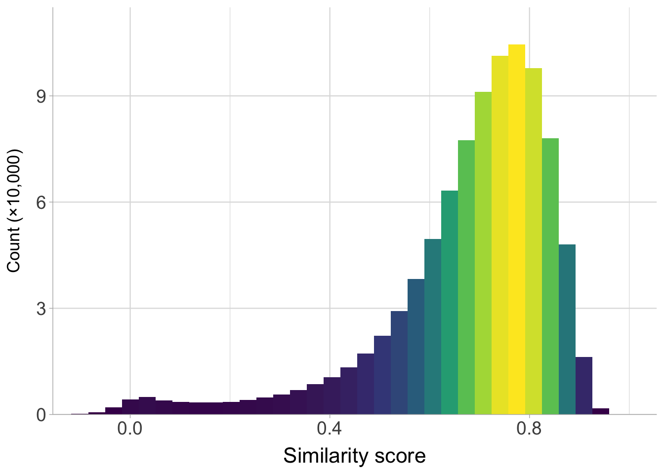
Plot the distribution of the similarity scores across all languages.
scores |>
  ggplot(aes(score)) +
  geom_histogram(aes(fill = after_stat(density)), bins = 40,
                 show.legend = F) +
  #geom_vline(xintercept = 0.38, color = "red3", linewidth = 0.5) +
  scale_fill_viridis_c() +
  scale_y_continuous(expand = expansion(mult = c(0, .1)),
                     label = scales::label_number(scale = 1/100000)) +
  scale_x_continuous(breaks = c(0, 0.4, 0.8)) +
  labs(y = expression("Count (\u00D710,000)"), x = "Similarity score") +
  coord_cartesian(xlim = c(-0.1, 1.0)) +
  theme(panel.grid.major.x = element_line(linewidth = 0.4),
        panel.grid.minor.x = element_line(linewidth = 0.2),
        panel.grid.major.y = element_line(linewidth = 0.4),
        axis.text.x = element_text(size=14),
        axis.text.y = element_text(size=14),
        axis.title.x = element_text(size=16),
        axis.title.y = element_text(size=13))
The next step require downloading speaker files from VoxCommunis Corpus.
# Replace the path below with the one on your own computer
spkr_dir <- "/Users/miaozhang/Research/VoxCommunis/VoxCommunis_Huggingface/speaker_files"
spkr_files <- list.files(spkr_dir, pattern = "*.tsv", full.names = T)

spkr_files <- map_dfr(spkr_files, \(x) read_tsv(x, col_select = c("path", "speaker_id"), show_col_types = FALSE))
spkr_files <- mutate(spkr_files, speaker_id = paste(str_extract(path, "(?<=voice_)[^_]+"), speaker_id, sep = "_"))
spkr_files <- rename(spkr_files, test = path)

spkr_files <- mutate(spkr_files, test = str_replace(test, ".mp3", ""))
scores <- mutate(scores, test = str_replace(test, ".wav", ""))

scores <- inner_join(scores, spkr_files, by = "test")
glimpse(scores)
## Rows: 8,497,101
## Columns: 6
## $ test            <chr> "common_voice_ab_27923256", "common_voice_ab_29441754"…
## $ enroll          <chr> "common_voice_ab_27923260.wav", "common_voice_ab_29441…
## $ score           <dbl> 0.4625, 0.5034, 0.6747, 0.2018, 0.0490, 0.6149, 0.0552…
## $ lang_code       <chr> "ab", "ab", "ab", "ab", "ab", "ab", "ab", "ab", "ab", …
## $ under_threshold <lgl> FALSE, FALSE, FALSE, TRUE, TRUE, FALSE, TRUE, TRUE, TR…
## $ speaker_id      <chr> "ab_5", "ab_6", "ab_14", "ab_7", "ab_8", "ab_8", "ab_9…
prop_under_threshold_by_lang <- scores |>
  summarize(prop_threshold = sum(under_threshold)/n(), .by = lang_code)
Evaluate how much the client IDs are affected by the heterogeneous speaker issue by looking into how many client IDs that contain recordings from multiple speakers there are.
speaker_id_impact <- scores |>
  summarize(n = n(), prop_threshold = sum(under_threshold)/n(), .by = speaker_id) |>
  mutate(affected = if_else(prop_threshold > 0, T, F),
         more_than_10 = if_else(prop_threshold > 0.10, T, F),
         lang = str_extract(speaker_id, "^[^_]+"))
n_affected_more_than_10 <- speaker_id_impact |>
  summarize(n_affected = sum(more_than_10),
            n_total = n(),
            perc = n_affected/n_total,
            .by = lang)

prop_more_than_100 <- scores |> summarize(n = n() + 1, .by = c(lang_code, speaker_id)) |>
  mutate(more_than_100 = if_else(n >= 100, T, F)) |>
  summarize(prop_more_than_100 = sum(more_than_100)/n(),
            n = n(),
            .by = lang_code)
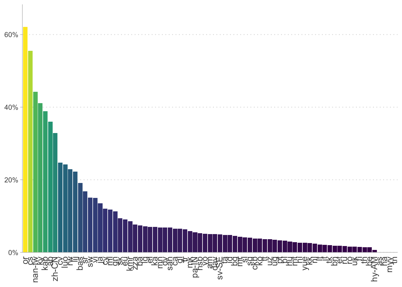
Plot the the degree to which client IDs and languages are affected.
# The proportion of files in each language with a score under the threshold
prop_under_threshold_by_lang |>
  ggplot(aes(reorder(lang_code, -prop_threshold), prop_threshold, fill = prop_threshold)) +
  geom_col() +
  scale_fill_viridis_c() +
  scale_y_continuous(labels = scales::percent_format(), lim = c(0,0.3),
                     expand = expansion(mult = c(0, .01))) +
  guides(fill = "none") +
  theme(axis.text.x = element_text(angle = 90, hjust = 1, vjust = 0.35, size = 11),
        axis.title.x = element_blank(),
        axis.title.y = element_blank(),
        axis.ticks.x = element_blank(),
        panel.grid.major.y = element_line(linetype = 3),
        legend.title = element_blank())

# The proportion of client IDs that have more than 10% of the associated recordings with a score lower than the threshold
ggplot(n_affected_more_than_10, aes(reorder(lang, desc(perc)), perc, fill = perc)) +
  geom_col() +
  scale_y_continuous(labels = scales::label_percent(), expand = expansion(mult = c(0, 0.1))) +
  scale_fill_viridis_c() +
  guides(fill = "none") +
  theme(axis.text.x = element_text(angle = 90, hjust = 1, vjust = 0.4, size = 11),
        axis.ticks.x = element_blank(),
        axis.title.x = element_blank(),
        axis.title.y = element_blank(),
        legend.title = element_blank(),
        panel.grid.major.y = element_line(linetype = 3))
Auditing result: round 1
Read in the auditing result from round 1.
audit_r1 <- read_csv("/Users/miaozhang/Documents/GitHub/CV_clientID_cleaning/audit_r1.csv") |>
  create_scoreBin() |>
  mutate(validation = factor(validation,
                             levels = c("Different Speaker", "Audio Quality Issue",
                                        "Missing Speech", "Not Sure", "Same Speaker")))
## Rows: 2048 Columns: 9
## ── Column specification ────────────────────────────────────────────────────────
## Delimiter: ","
## chr (5): test, enroll, lang, validation, score_bin
## dbl (4): score, up_votes, down_votes, speaker_id
##
## ℹ Use `spec()` to retrieve the full column specification for this data.
## ℹ Specify the column types or set `show_col_types = FALSE` to quiet this message.
glimpse(audit_r1)
## Rows: 2,048
## Columns: 9
## $ test       <chr> "common_voice_ab_29496822.mp3", "common_voice_ab_29537063.m…
## $ enroll     <chr> "common_voice_ab_29550540.mp3", "common_voice_ab_29550540.m…
## $ score      <dbl> 0.1851, 0.2400, 0.2835, 0.4160, 0.4256, 0.1969, 0.0090, 0.1…
## $ lang       <chr> "ab", "ab", "ab", "ab", "ab", "ab", "ab", "ab", "ab", "ab",…
## $ up_votes   <dbl> 2, 2, 2, 3, 2, 2, 2, 2, 2, 2, 2, 2, 2, 2, 2, 2, 2, 2, 2, 2,…
## $ down_votes <dbl> 0, 0, 0, 0, 0, 0, 0, 0, 0, 0, 0, 0, 0, 0, 0, 0, 0, 0, 0, 0,…
## $ speaker_id <dbl> 367, 367, 367, 324, 266, 367, 355, 247, 364, 367, 364, 353,…
## $ validation <fct> Different Speaker, Different Speaker, Different Speaker, Di…
## $ score_bin  <fct> < 0.2, < 0.3, < 0.3, < 0.5, < 0.5, < 0.2, < 0.1, < 0.2, < 0…
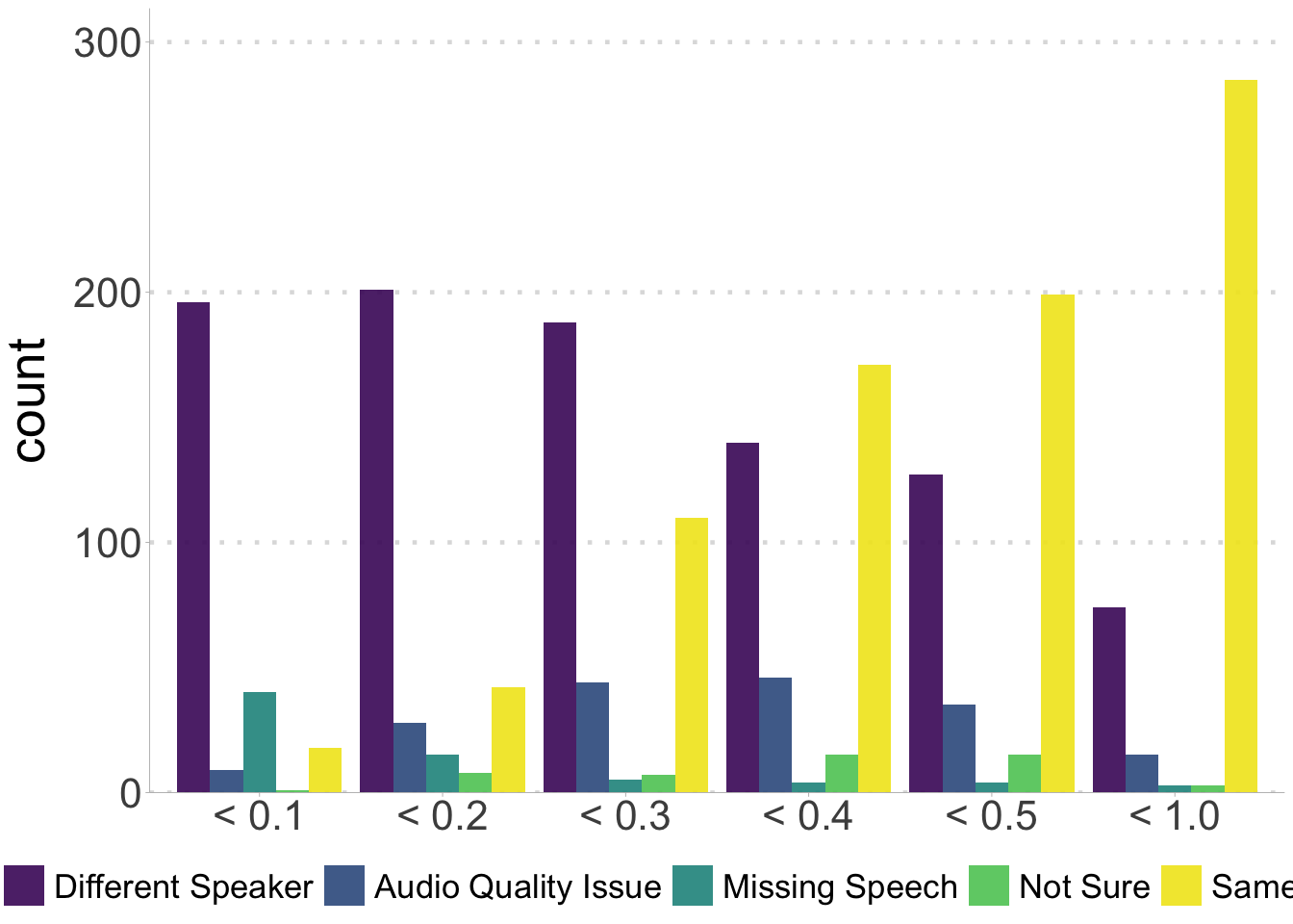
Plot the round 1 results.
ggplot(audit_r1, aes(x = score_bin, fill = validation)) +
  stat_count(position = "dodge") +
  scale_fill_viridis_d(end = 0.98, begin = 0.05, alpha = 0.9) +
  scale_y_continuous(expand = expansion(mult = c(0, 0.1))) +
  theme_ggdist(base_size = 6.5) +
  theme(axis.title.x = element_blank(),
        panel.grid.major.y = element_line(linetype = 3, linewidth = 0.8),
        axis.text = element_text(size = 16),
        axis.title.y = element_text(size = 20),
        legend.text = element_text(size = 13),
        legend.position = "bottom",
        legend.title = element_blank())
Auditing result: round 1
Get the round 2 data.
audit_r2 <- read_csv("/Users/miaozhang/Documents/GitHub/CV_clientID_cleaning/audit_r2.csv") |> create_scoreBin()
## Rows: 150 Columns: 18
## ── Column specification ────────────────────────────────────────────────────────
## Delimiter: ","
## chr (14): lang, test, enroll, person1, validation1, person2, validation2, pe...
## dbl  (4): score, up_votes, down_votes, speaker_id
##
## ℹ Use `spec()` to retrieve the full column specification for this data.
## ℹ Specify the column types or set `show_col_types = FALSE` to quiet this message.
glimpse(audit_r2)
## Rows: 150
## Columns: 18
## $ lang        <chr> "ab", "am", "am", "ba", "ba", "bas", "bas", "bas", "bas", …
## $ test        <chr> "common_voice_ab_29535966.mp3", "common_voice_am_37890165.…
## $ enroll      <chr> "common_voice_ab_29550540.mp3", "common_voice_am_37952755.…
## $ score       <dbl> 0.2567, 0.3594, 0.4269, 0.2330, 0.4308, 0.1913, 0.4854, 0.…
## $ up_votes    <dbl> 2, 2, 2, 2, 2, 2, 2, 2, 2, 3, 2, 2, 3, 3, 2, 2, 2, 2, 2, 2…
## $ down_votes  <dbl> 0, 0, 0, 0, 0, 0, 0, 0, 0, 0, 0, 0, 0, 0, 0, 0, 0, 0, 0, 0…
## $ speaker_id  <dbl> 367, 19, 19, 807, 884, 47, 48, 48, 48, 8210, 6455, 7154, 3…
## $ person1     <chr> "Annotator1", "Annotator1", "Annotator1", "Annotator1", "A…
## $ validation1 <chr> "Different Speaker", "Same Speaker", "Same Speaker", "Same…
## $ person2     <chr> "Annotator2", "Annotator2", "Annotator2", "Annotator2", "A…
## $ validation2 <chr> "Different Speaker", "Same Speaker", "Same Speaker", "Same…
## $ person3     <chr> "Annotator3", "Annotator3", "Annotator3", "Annotator3", "A…
## $ validation3 <chr> "Different Speaker", "Same Speaker", "Same Speaker", "Same…
## $ person4     <chr> "Annotator4", "Annotator4", "Annotator4", "Annotator4", "A…
## $ validation4 <chr> "Different Speaker", "Same Speaker", "Same Speaker", "Same…
## $ person5     <chr> "Annotator5", "Annotator5", "Annotator5", "Annotator5", "A…
## $ validation5 <chr> "Different Speaker", "Different Speaker", "Same Speaker", …
## $ score_bin   <fct> < 0.3, < 0.4, < 0.5, < 0.3, < 0.5, < 0.2, < 0.5, < 0.5, < …
Calculate the Fleiss’ Kappa.
kappa_dat <- audit_r2[, colnames(audit_r2) %in% c("validation1", "validation2", "validation3", "validation4", "validation5")]
kappam.fleiss(kappa_dat)
##  Fleiss' Kappa for m Raters
##
##  Subjects = 150
##    Raters = 5
##     Kappa = 0.446
##
##         z = 21.6
##   p-value = 0
Fit a GLMER model to evaluate the threshold to reject same speaker hypothesis.
audit_r2_long <- audit_r2 %>% pivot_longer(cols = starts_with("person"),
                             names_to = ("person"),
                             values_to = "name") %>%
  pivot_longer(cols = starts_with("validation"),
               names_to = ("validation"),
               values_to = "val")
audit_r2_long <- subset(audit_r2_long, name == "Annotator1" & validation == "validation1" |
                   name == "Annotator2" & validation == "validation2" |
                   name == "Annotator3" & validation == "validation3" |
                   name == "Annotator4" & validation == "validation4" |
                   name == "Annotator5" & validation == "validation5")
glimpse(audit_r2_long)
## Rows: 750
## Columns: 12
## $ lang       <chr> "ab", "ab", "ab", "ab", "ab", "am", "am", "am", "am", "am",…
## $ test       <chr> "common_voice_ab_29535966.mp3", "common_voice_ab_29535966.m…
## $ enroll     <chr> "common_voice_ab_29550540.mp3", "common_voice_ab_29550540.m…
## $ score      <dbl> 0.2567, 0.2567, 0.2567, 0.2567, 0.2567, 0.3594, 0.3594, 0.3…
## $ up_votes   <dbl> 2, 2, 2, 2, 2, 2, 2, 2, 2, 2, 2, 2, 2, 2, 2, 2, 2, 2, 2, 2,…
## $ down_votes <dbl> 0, 0, 0, 0, 0, 0, 0, 0, 0, 0, 0, 0, 0, 0, 0, 0, 0, 0, 0, 0,…
## $ speaker_id <dbl> 367, 367, 367, 367, 367, 19, 19, 19, 19, 19, 19, 19, 19, 19…
## $ score_bin  <fct> < 0.3, < 0.3, < 0.3, < 0.3, < 0.3, < 0.4, < 0.4, < 0.4, < 0…
## $ person     <chr> "person1", "person2", "person3", "person4", "person5", "per…
## $ name       <chr> "Annotator1", "Annotator2", "Annotator3", "Annotator4", "An…
## $ validation <chr> "validation1", "validation2", "validation3", "validation4",…
## $ val        <chr> "Different Speaker", "Different Speaker", "Different Speake…
samediff_all <- subset(audit_r2_long, val %in% c("Same Speaker","Different Speaker"))
samediff_all$nVal <- ifelse(samediff_all$val == "Same Speaker", 1, 0)
mod <- glmer(nVal ~ score + (1 | person) + (0 + score | person), family = "binomial", data = samediff_all)
Get the threshold.
threshold <- -fixef(mod)[1]/fixef(mod)[2]
threshold
## (Intercept)
##   0.3874009
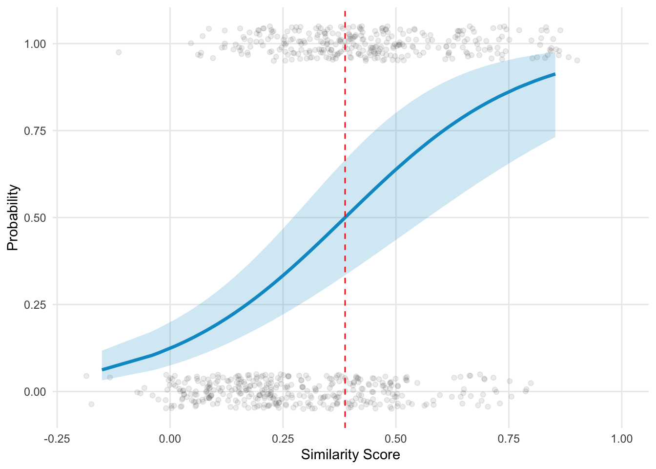
Plot the model result.
samediff_all$predicted <- predict(mod, type = "response", re.form = NA)
samediff_all$predicted_person <- predict(mod, type = "response")
preds <- ggpredict(mod, terms = "score[all]", interval = "confidence")
## You are calculating adjusted predictions on the population-level (i.e.
##   `type = "fixed"`) for a *generalized* linear mixed model.
##   This may produce biased estimates due to Jensen's inequality. Consider
##   setting `bias_correction = TRUE` to correct for this bias.
##   See also the documentation of the `bias_correction` argument.
ggplot(samediff_all, aes(x = score, y = nVal)) +
  geom_jitter(alpha = 0.08, width = 0.05, height = 0.05) +
  # Confidence interval ribbon
  geom_ribbon(data = preds, aes(x = x, ymin = conf.low, ymax = conf.high),
              fill = "deepskyblue3", alpha = 0.2, inherit.aes = FALSE) +
  # Model prediction line
  geom_line(data = preds, aes(x = x, y = predicted),
            color = "deepskyblue3", size = 1.2, inherit.aes = FALSE) +
  scale_x_continuous(limits = c(-0.2, 1)) +
  labs(x = "Similarity Score", y = "Probability") +
  geom_vline(xintercept = threshold, linetype = "dashed", color = "red") +
  theme_minimal() +
  theme(panel.grid.minor = element_blank())
## Warning: Using `size` aesthetic for lines was deprecated in ggplot2 3.4.0.
## ℹ Please use `linewidth` instead.
## This warning is displayed once every 8 hours.
## Call `lifecycle::last_lifecycle_warnings()` to see where this warning was
## generated.