Introduction
This page is intended to reproduce the results and visualizations from the paper Zhang, M., Farhadipour, A., Baker, A., Ma, J., Pricop, B., Chodroff, E. (2025) Quantifying and Reducing Speaker Heterogeneity within the Common Voice Corpus for Phonetic Analysis. Proc. Interspeech 2025, 3933-3937, doi: 10.21437/Interspeech.2025-2027.
This paper addresses the problem of speaker heterogeneity in the Mozilla Common Voice corpus, where a single “client ID” may include recordings from multiple speakers, complicating phonetic analysis and speech technology development. We use ResNet-293-based speaker embeddings to compute similarity scores between utterances within the same client ID and then design a speaker discrimination task to determine an optimal similarity threshold. Through large-scale evaluation across 76 languages, we identify a threshold of 0.354 that effectively reduces speaker heterogeneity while minimizing data loss (averaging 3.5% per language).
How to use this script
There are several data files you need to download from the repo to run this script yourself.
Similarity scores
Load the similarity score file into R and obtain some descriptive stats.
# Define the column names of the similarity score file.
col_names <- c("test", "enroll", "score")

# Replace the file path with the one on your computer
path2scores <- "/Users/miaozhang/Research/VoxCommunis/VoxCommunis_Huggingface/similarity_scores_interspeech2025.txt"
scores <- read_delim(path2scores, col_names = col_names, show_col_types = FALSE, delim = " ")

# Use the threshold from our paper
threshold = 0.354

# Get the language codes and check if the file has a score under the threshold
scores <- scores |> mutate(lang_code = str_extract(enroll, "(?<=voice_)[^_]+"), # Get the languages
                           under_threshold = if_else(score < threshold, T, F))
glimpse(scores)
## Rows: 9,204,867
## Columns: 5
## $ test            <chr> "common_voice_ab_27923256.wav", "common_voice_ab_29441…
## $ enroll          <chr> "common_voice_ab_27923260.wav", "common_voice_ab_29441…
## $ score           <dbl> 0.4625, 0.5034, 0.6747, 0.2018, 0.0490, 0.6149, 0.0552…
## $ lang_code       <chr> "ab", "ab", "ab", "ab", "ab", "ab", "ab", "ab", "ab", …
## $ under_threshold <lgl> FALSE, FALSE, FALSE, TRUE, TRUE, FALSE, TRUE, FALSE, T…
# Get some summary of the similarity scores
summary(scores$score)
##    Min. 1st Qu.  Median    Mean 3rd Qu.    Max.
## -0.3132  0.6164  0.7196  0.6795  0.7951  1.0000
scores_by_lang <- scores |>
  group_by(lang_code) |>
  summarise(q1 = quantile(score, 0.25),
            median = median(score),
            q3 = quantile(score, 0.75))
summary(scores_by_lang$q1)
##    Min. 1st Qu.  Median    Mean 3rd Qu.    Max.
##  0.3687  0.5857  0.6347  0.6191  0.6662  0.7533
summary(scores_by_lang$q3)
##    Min. 1st Qu.  Median    Mean 3rd Qu.    Max.
##  0.5964  0.7501  0.7849  0.7766  0.8071  0.8691
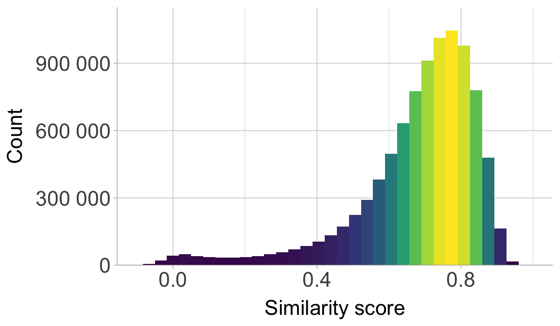
Plot the distribution of the similarity scores.
scores |>
  ggplot(aes(score)) +
  geom_histogram(aes(fill = after_stat(density)), bins = 40,
                 show.legend = F) +
  scale_fill_viridis_c() +
  scale_y_continuous(expand = expansion(mult = c(0, .1)),
                     label = scales::label_number(scale = 1)) +
  scale_x_continuous(breaks = c(0, 0.4, 0.8)) +
  labs(y = expression("Count"), x = "Similarity score") +
  coord_cartesian(xlim = c(-0.1, 1.0)) +
  theme(panel.grid.major.x = element_line(linewidth = 0.4),
        panel.grid.minor.x = element_line(linewidth = 0.2),
        panel.grid.major.y = element_line(linewidth = 0.4),
        axis.text.x = element_text(size=16),
        axis.text.y = element_text(size=16),
        axis.title.x = element_text(size=16),
        axis.title.y = element_text(size=16))
Then load the speaker files.
# Replace the path below with the one on your own computer
spkr_dir <- "/Users/miaozhang/Research/VoxCommunis/VoxCommunis_Huggingface/speaker_files"
spkr_files <- list.files(spkr_dir, pattern = "*.tsv", full.names = T)

spkr_files <- map_dfr(spkr_files, \(x) read_tsv(x, col_select = c("path", "speaker_id"), show_col_types = FALSE))

# Unify the extension in both datasets
spkr_files <- mutate(spkr_files,
                     speaker_id = paste(str_extract(path, "(?<=voice_)[^_]+"), speaker_id, sep = "_")) |>
  rename(test = path) |>
  mutate(test = str_replace(test, ".mp3", ""))
scores <- mutate(scores, test = str_replace(test, ".wav", ""))

# join the two datasets together
scores <- inner_join(scores, spkr_files, by = "test")
glimpse(scores)
## Rows: 9,204,456
## Columns: 6
## $ test            <chr> "common_voice_ab_27923256", "common_voice_ab_29441754"…
## $ enroll          <chr> "common_voice_ab_27923260.wav", "common_voice_ab_29441…
## $ score           <dbl> 0.4625, 0.5034, 0.6747, 0.2018, 0.0490, 0.6149, 0.0552…
## $ lang_code       <chr> "ab", "ab", "ab", "ab", "ab", "ab", "ab", "ab", "ab", …
## $ under_threshold <lgl> FALSE, FALSE, FALSE, TRUE, TRUE, FALSE, TRUE, FALSE, T…
## $ speaker_id      <chr> "ab_5", "ab_6", "ab_14", "ab_7", "ab_8", "ab_8", "ab_9…
# Get the propotion of files under the threshold in each language
prop_under_threshold_by_lang <- scores |>
  summarize(prop_threshold = sum(under_threshold)/n(), .by = lang_code)
Evaluate to what extent the client IDs are affected by speaker heterogeneity by looking into the number of client IDs that contain recordings from multiple speakers.
# Summarize by speaker_id: compute number of files (n) and proportion under threshold
speaker_id_impact <- scores |>
  summarize(
    n = n() + 1,
    prop_threshold = sum(under_threshold) / (n() + 1),
    .by = speaker_id
  ) |>
  mutate(
    affected = if_else(prop_threshold > 0, T, F),          # Check if any of the recordings under the client ID are from a different speaker
    more_than_10 = if_else(prop_threshold > 0.10, T, F),  # Check if more than 10% of the recordings under the client ID are from a different speaker
    lang = str_extract(speaker_id, "^[^_]+")
  )

# Count how many speakers are affected by >10% under threshold, per language
n_affected_more_than_10 <- speaker_id_impact |>
  summarize(
    n_affected = sum(more_than_10),         # number of speakers with >10% affected
    n_total = n(),                          # total speakers
    perc = n_affected / n_total,            # proportion affected
    .by = lang
  )

# For each speaker, count if they have more than 100 files
prop_more_than_100 <- scores |>
  summarize(n = n() + 1, .by = c(lang_code, speaker_id)) |>
  mutate(more_than_100 = if_else(n >= 100, T, F)) |>   # flag speakers with >= 100 files
  summarize(
    prop_more_than_100 = sum(more_than_100) / n(),     # proportion of speakers with >= 100 files
    n = n(),                                          # total speakers
    .by = lang_code
  )

# Check the distribution of prop_threshold by language
print("Proportion of files under the threshold by language:")
## [1] "Proportion of files under the threshold by language:"
print(summary(prop_under_threshold_by_lang$prop_threshold))
##      Min.   1st Qu.    Median      Mean   3rd Qu.      Max.
## 0.0008031 0.0078664 0.0161182 0.0351913 0.0463015 0.2179372
# Count speakers under various cutoff conditions
print(paste("Languages with <10% under threshold:",
            nrow(subset(prop_under_threshold_by_lang, prop_threshold < 0.1))))
## [1] "Languages with <10% under threshold: 70"
print(paste("Number of Client IDs with <10% under threshold: ",
            nrow(subset(speaker_id_impact, prop_threshold < 0.1))))
## [1] "Number of Client IDs with <10% under threshold: 113735"
print(paste("Proportion of client IDs <10% under threshold:",
            round(nrow(subset(speaker_id_impact, prop_threshold < 0.1)) /
                    nrow(speaker_id_impact), 3)))
## [1] "Proportion of client IDs <10% under threshold: 0.919"
# Summarize affected speakers by language and whether >10% affected
affected_ids <- speaker_id_impact |>
  group_by(lang, more_than_10) |>
  summarise(greaterThan10 = n()) |>          # count speakers per lang × condition
  pivot_wider(names_from = more_than_10, values_from = greaterThan10) |>
  rename("good" = `FALSE`,                   # "good" = speakers not badly affected
         "bad" = `TRUE`) |>                  # "bad" = speakers with >10% data affected
  mutate(
    bad = ifelse(is.na(bad), 0, bad),        # replace NA with 0 for langs with no "bad" speakers
    total = sum(good + bad),                 # total speakers per language
    prop = bad / total                       # proportion of "bad" speakers
  )
## `summarise()` has grouped output by 'lang'. You can override using the
## `.groups` argument.
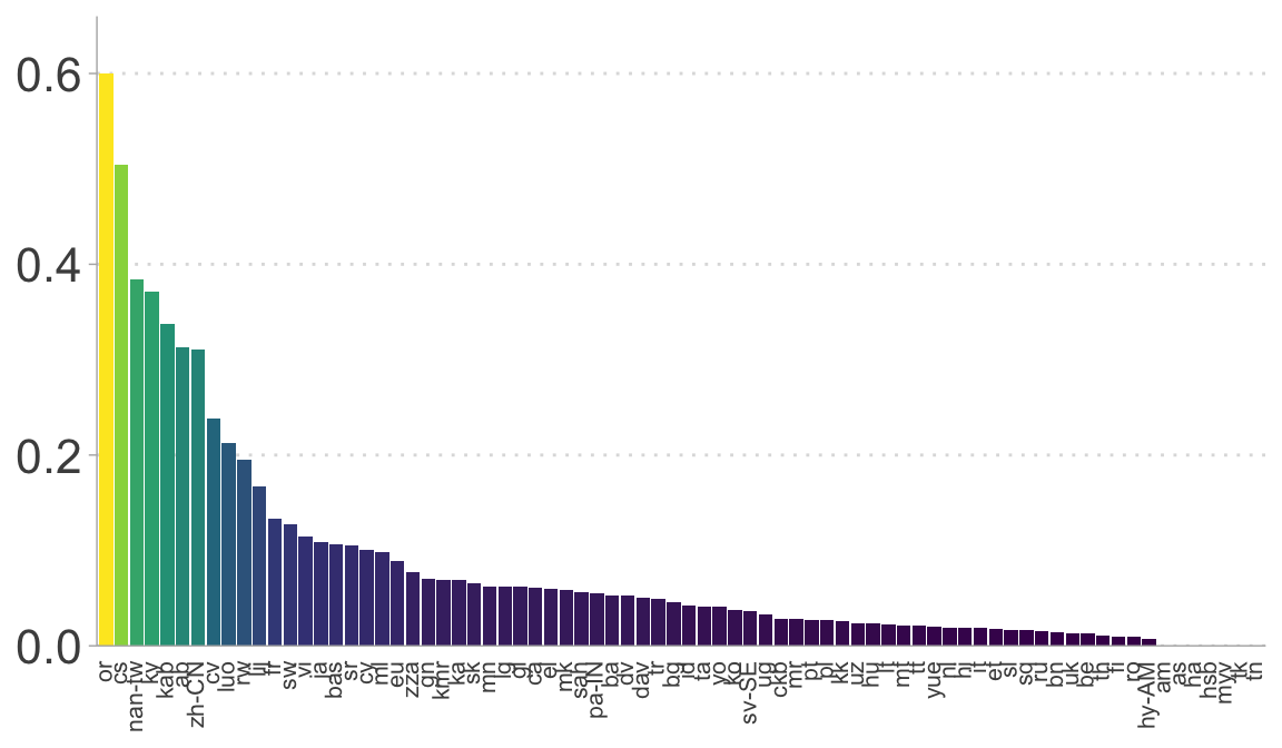
# Distribution of bad-speaker proportions across languages
print("The proportion of client IDs that contain different speaker's voices in more than 10% of the associated recordings")
## [1] "The proportion of client IDs that contain different speaker's voices in more than 10% of the associated recordings"
summary(affected_ids$prop)
##    Min. 1st Qu.  Median    Mean 3rd Qu.    Max.
## 0.00000 0.01891 0.04356 0.08414 0.09144 0.60000
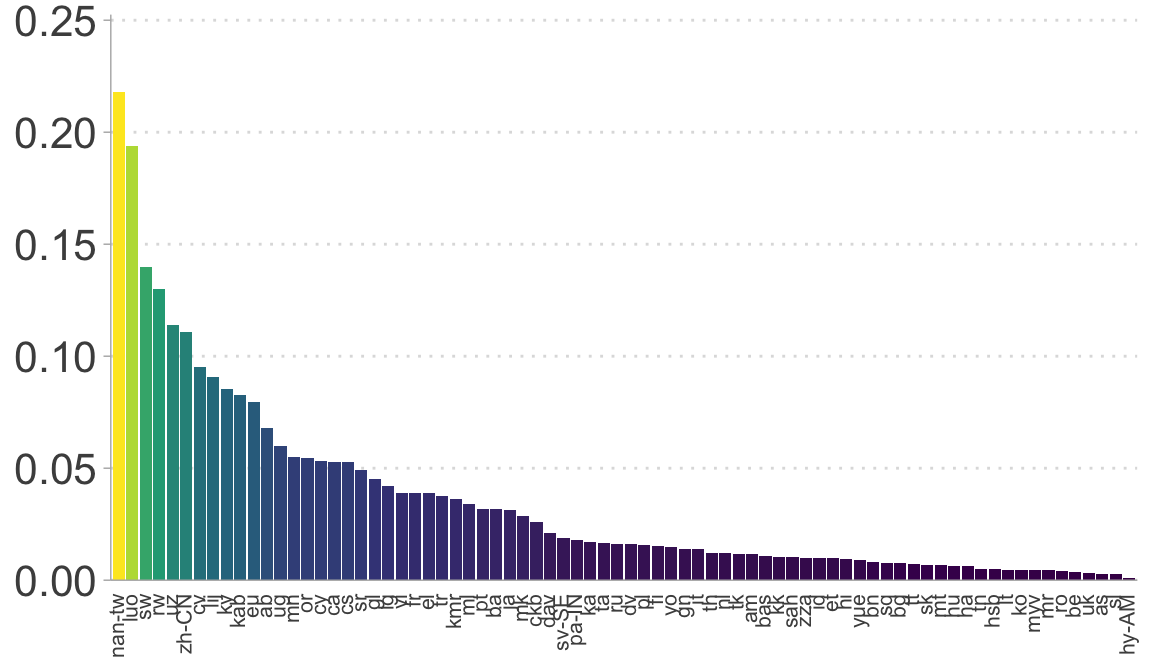
Plot the the degree to which client IDs and languages are affected.
# The proportion of files in each language with a score under the threshold
prop_under_threshold_by_lang |>
  ggplot(aes(reorder(lang_code, -prop_threshold), prop_threshold, fill = prop_threshold)) +
  geom_col() +
  scale_fill_viridis_c() +
  scale_y_continuous(lim = c(0,0.25),
                     expand = expansion(mult = c(0, .01))) +
  guides(fill = "none") +
  #ylab("Prop. utterances") +
  theme(axis.text.x = element_text(angle = 90, hjust = 1, vjust = 0.35, size = 8),
        axis.title.x = element_blank(),
        axis.title.y = element_blank(),
        #axis.title.y = element_text(size = 16),
        axis.text.y = element_text(size = 16),
        axis.ticks.x = element_blank(),
        panel.grid.major.y = element_line(linetype = 3),
        legend.title = element_blank())
# The proportion of client IDs that have more than 10% of the associated recordings with a score lower than the threshold
ggplot(n_affected_more_than_10, aes(reorder(lang, desc(perc)), perc, fill = perc)) +
  geom_col() +
  scale_y_continuous(expand = expansion(mult = c(0, 0.1))) +
  scale_fill_viridis_c() +
  guides(fill = "none") +
  #ylab("Prop. client IDs") +
  theme(axis.text.x = element_text(angle = 90, hjust = 1, vjust = 0.35, size = 8),
        axis.title.x = element_blank(),
        axis.title.y = element_blank(),
        #axis.title.y = element_text(size = 16),
        axis.text.y = element_text(size = 16),
        axis.ticks.x = element_blank(),
        legend.title = element_blank(),
        panel.grid.major.y = element_line(linetype = 3))
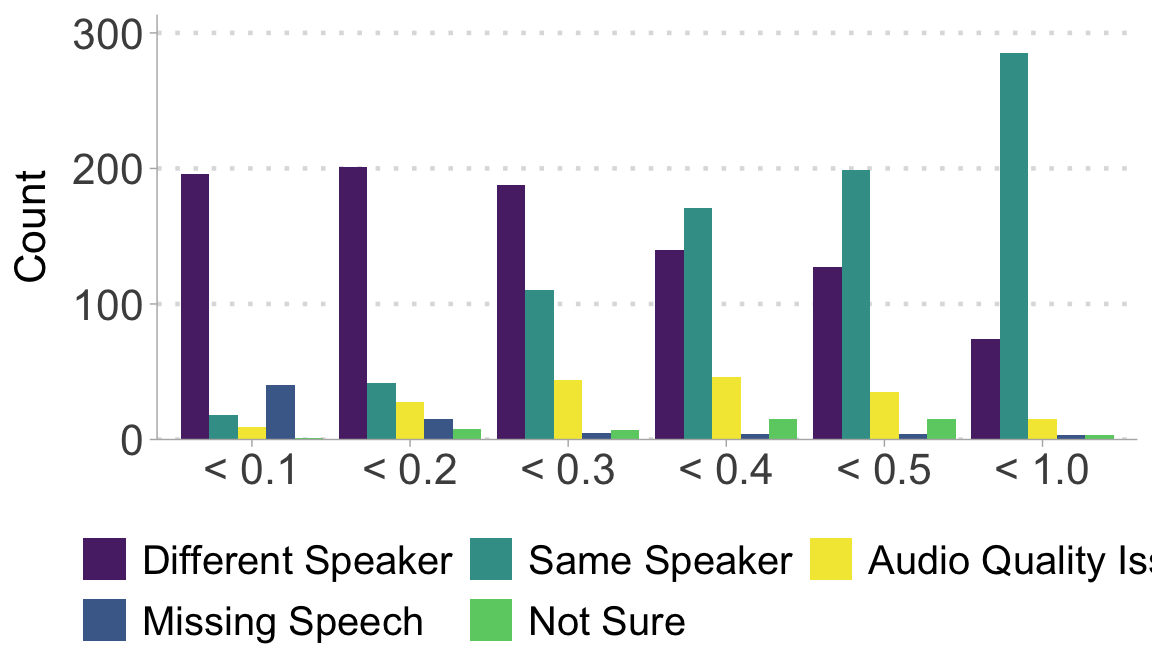
Auditing result: round 1
Read in the auditing result from round 1.
# load the first round audit result
audit_r1 <- read_csv("~/Documents/GitHub/miaozhang/static/papers_slides/audit_r1.csv") |>
  create_scoreBin() |>
  mutate(validation = factor(validation,
                             levels = c("Different Speaker",
                                        "Same Speaker",
                                        "Audio Quality Issue",
                                        "Missing Speech",
                                        "Not Sure"
                                        )))
## Rows: 2048 Columns: 9
## ── Column specification ────────────────────────────────────────────────────────
## Delimiter: ","
## chr (5): test, enroll, lang, validation, score_bin
## dbl (4): score, up_votes, down_votes, speaker_id
##
## ℹ Use `spec()` to retrieve the full column specification for this data.
## ℹ Specify the column types or set `show_col_types = FALSE` to quiet this message.
glimpse(audit_r1)
## Rows: 2,048
## Columns: 9
## $ test       <chr> "common_voice_ab_29496822.mp3", "common_voice_ab_29537063.m…
## $ enroll     <chr> "common_voice_ab_29550540.mp3", "common_voice_ab_29550540.m…
## $ score      <dbl> 0.1851, 0.2400, 0.2835, 0.4160, 0.4256, 0.1969, 0.0090, 0.1…
## $ lang       <chr> "ab", "ab", "ab", "ab", "ab", "ab", "ab", "ab", "ab", "ab",…
## $ up_votes   <dbl> 2, 2, 2, 3, 2, 2, 2, 2, 2, 2, 2, 2, 2, 2, 2, 2, 2, 2, 2, 2,…
## $ down_votes <dbl> 0, 0, 0, 0, 0, 0, 0, 0, 0, 0, 0, 0, 0, 0, 0, 0, 0, 0, 0, 0,…
## $ speaker_id <dbl> 367, 367, 367, 324, 266, 367, 355, 247, 364, 367, 364, 353,…
## $ validation <fct> Different Speaker, Different Speaker, Different Speaker, Di…
## $ score_bin  <fct> < 0.2, < 0.3, < 0.3, < 0.5, < 0.5, < 0.2, < 0.1, < 0.2, < 0…
Plot the round 1 results.
ggplot(audit_r1, aes(x = score_bin, fill = validation)) +
  stat_count(position = "dodge") +
  scale_fill_manual(values = c("#5a2b75", "#3d9e96", "#f3e740", "#4a6b99", "#6bcd72")) +
  scale_y_continuous(expand = expansion(mult = c(0, 0.1))) +
  #theme_ggdist(base_size = 6.5) +
  ylab("Count") +
  guides(fill=guide_legend(nrow=2,byrow=TRUE)) +
  theme(axis.title.x = element_blank(),
        panel.grid.major.y = element_line(linetype = 3, linewidth = 0.8),
        axis.text = element_text(size = 16),
        axis.title.y = element_text(size = 16),
        legend.text = element_text(size = 15),
        legend.position = "bottom",
        legend.title = element_blank())
Auditing result: round 1
Get the round 2 data.
audit_r2 <- read_csv("~/Documents/GitHub/miaozhang/static/papers_slides/audit_r2.csv") |> create_scoreBin()
## Rows: 150 Columns: 18
## ── Column specification ────────────────────────────────────────────────────────
## Delimiter: ","
## chr (14): lang, test, enroll, person1, validation1, person2, validation2, pe...
## dbl  (4): score, up_votes, down_votes, speaker_id
##
## ℹ Use `spec()` to retrieve the full column specification for this data.
## ℹ Specify the column types or set `show_col_types = FALSE` to quiet this message.
glimpse(audit_r2)
## Rows: 150
## Columns: 18
## $ lang        <chr> "ab", "am", "am", "ba", "ba", "bas", "bas", "bas", "bas", …
## $ test        <chr> "common_voice_ab_29535966.mp3", "common_voice_am_37890165.…
## $ enroll      <chr> "common_voice_ab_29550540.mp3", "common_voice_am_37952755.…
## $ score       <dbl> 0.2567, 0.3594, 0.4269, 0.2330, 0.4308, 0.1913, 0.4854, 0.…
## $ up_votes    <dbl> 2, 2, 2, 2, 2, 2, 2, 2, 2, 3, 2, 2, 3, 3, 2, 2, 2, 2, 2, 2…
## $ down_votes  <dbl> 0, 0, 0, 0, 0, 0, 0, 0, 0, 0, 0, 0, 0, 0, 0, 0, 0, 0, 0, 0…
## $ speaker_id  <dbl> 367, 19, 19, 807, 884, 47, 48, 48, 48, 8210, 6455, 7154, 3…
## $ person1     <chr> "Annotator1", "Annotator1", "Annotator1", "Annotator1", "A…
## $ validation1 <chr> "Different Speaker", "Same Speaker", "Same Speaker", "Same…
## $ person2     <chr> "Annotator2", "Annotator2", "Annotator2", "Annotator2", "A…
## $ validation2 <chr> "Different Speaker", "Same Speaker", "Same Speaker", "Same…
## $ person3     <chr> "Annotator3", "Annotator3", "Annotator3", "Annotator3", "A…
## $ validation3 <chr> "Different Speaker", "Same Speaker", "Same Speaker", "Same…
## $ person4     <chr> "Annotator4", "Annotator4", "Annotator4", "Annotator4", "A…
## $ validation4 <chr> "Different Speaker", "Same Speaker", "Same Speaker", "Same…
## $ person5     <chr> "Annotator5", "Annotator5", "Annotator5", "Annotator5", "A…
## $ validation5 <chr> "Different Speaker", "Different Speaker", "Same Speaker", …
## $ score_bin   <fct> < 0.3, < 0.4, < 0.5, < 0.3, < 0.5, < 0.2, < 0.5, < 0.5, < …
Calculate the Fleiss’ Kappa.
kappa_dat <- audit_r2[, colnames(audit_r2) %in% c("validation1", "validation2", "validation3", "validation4", "validation5")]
kappa_result <- kappam.fleiss(kappa_dat)
print(paste0("The Fleiss' Kappa = ", round(kappa_result$value, 2)))
## [1] "The Fleiss' Kappa = 0.45"
Fit a GLMM model to evaluate a threshold for rejecting same-speaker hypothesis.
audit_r2_long <- audit_r2 |>
  pivot_longer(cols = starts_with("person"), names_to = ("person"), values_to = "name") |>
  pivot_longer(cols = starts_with("validation"), names_to = ("validation"), values_to = "val") |>
  filter(name == "Annotator1" & validation == "validation1" |
           name == "Annotator2" & validation == "validation2" |
           name == "Annotator3" & validation == "validation3" |
           name == "Annotator4" & validation == "validation4" |
           name == "Annotator5" & validation == "validation5")
glimpse(audit_r2_long)
## Rows: 750
## Columns: 12
## $ lang       <chr> "ab", "ab", "ab", "ab", "ab", "am", "am", "am", "am", "am",…
## $ test       <chr> "common_voice_ab_29535966.mp3", "common_voice_ab_29535966.m…
## $ enroll     <chr> "common_voice_ab_29550540.mp3", "common_voice_ab_29550540.m…
## $ score      <dbl> 0.2567, 0.2567, 0.2567, 0.2567, 0.2567, 0.3594, 0.3594, 0.3…
## $ up_votes   <dbl> 2, 2, 2, 2, 2, 2, 2, 2, 2, 2, 2, 2, 2, 2, 2, 2, 2, 2, 2, 2,…
## $ down_votes <dbl> 0, 0, 0, 0, 0, 0, 0, 0, 0, 0, 0, 0, 0, 0, 0, 0, 0, 0, 0, 0,…
## $ speaker_id <dbl> 367, 367, 367, 367, 367, 19, 19, 19, 19, 19, 19, 19, 19, 19…
## $ score_bin  <fct> < 0.3, < 0.3, < 0.3, < 0.3, < 0.3, < 0.4, < 0.4, < 0.4, < 0…
## $ person     <chr> "person1", "person2", "person3", "person4", "person5", "per…
## $ name       <chr> "Annotator1", "Annotator2", "Annotator3", "Annotator4", "An…
## $ validation <chr> "validation1", "validation2", "validation3", "validation4",…
## $ val        <chr> "Different Speaker", "Different Speaker", "Different Speake…
samediff_all <- audit_r2_long |>
  filter(val %in% c("Same Speaker","Different Speaker")) |>
  mutate(nVal = ifelse(val == "Same Speaker", 1, 0))
mod <- glmer(nVal ~ score + (1 | person) + (0 + score | person) + (1 | lang) + (0 + score | lang), family = "binomial", data = samediff_all)
summary(mod)
## Generalized linear mixed model fit by maximum likelihood (Laplace
##   Approximation) [glmerMod]
##  Family: binomial  ( logit )
## Formula: nVal ~ score + (1 | person) + (0 + score | person) + (1 | lang) +
##     (0 + score | lang)
##    Data: samediff_all
##
##      AIC      BIC   logLik deviance df.resid
##    666.2    693.4   -327.1    654.2      676
##
## Scaled residuals:
##     Min      1Q  Median      3Q     Max
## -3.4124 -0.4147 -0.1505  0.4724  3.2366
##
## Random effects:
##  Groups   Name        Variance Std.Dev.
##  lang     score       17.0605  4.1304
##  lang.1   (Intercept)  3.0314  1.7411
##  person   score        5.3859  2.3208
##  person.1 (Intercept)  0.5061  0.7114
## Number of obs: 682, groups:  lang, 61; person, 5
##
## Fixed effects:
##             Estimate Std. Error z value Pr(>|z|)
## (Intercept)  -2.8930     0.5499  -5.261 1.43e-07 ***
## score         8.1719     1.6040   5.095 3.50e-07 ***
## ---
## Signif. codes:  0 '***' 0.001 '**' 0.01 '*' 0.05 '.' 0.1 ' ' 1
##
## Correlation of Fixed Effects:
##       (Intr)
## score -0.436
Get the threshold.
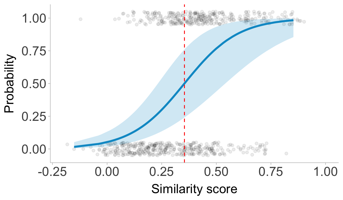
threshold <- -fixef(mod)[1]/fixef(mod)[2]
print(paste0("The threshold is ", round(threshold, 3)))
## [1] "The threshold is 0.354"
Plot the model result.
samediff_all$predicted <- predict(mod, type = "response", re.form = NA)
samediff_all$predicted_person <- predict(mod, type = "response")
preds <- ggpredict(mod, terms = "score[all]", interval = "confidence")
## You are calculating adjusted predictions on the population-level (i.e.
##   `type = "fixed"`) for a *generalized* linear mixed model.
##   This may produce biased estimates due to Jensen's inequality. Consider
##   setting `bias_correction = TRUE` to correct for this bias.
##   See also the documentation of the `bias_correction` argument.
ggplot(samediff_all, aes(x = score, y = nVal)) +
  geom_jitter(alpha = 0.08, width = 0.05, height = 0.05) +
  # Confidence interval ribbon
  geom_ribbon(data = preds, aes(x = x, ymin = conf.low, ymax = conf.high),
              fill = "deepskyblue3", alpha = 0.2, inherit.aes = FALSE) +
  # Model prediction line
  geom_line(data = preds, aes(x = x, y = predicted),
            color = "deepskyblue3", linewidth = 1.2, inherit.aes = FALSE) +
  scale_x_continuous(limits = c(-0.2, 1)) +
  labs(x = "Similarity score", y = "Probability") +
  geom_vline(xintercept = threshold, linetype = "dashed", color = "red") +
  theme(panel.grid.minor = element_blank(),
        axis.text.y = element_text(size = 16),
        axis.title.y = element_text(size = 16),
        axis.text.x = element_text(size = 16),
        axis.title.x = element_text(size = 16))